Exact Evaluation
Exact Evaluation
Exact Versus Subjective
For example, if the answer to a multiple-choice question is A and you pick B, your answer is wrong. There's no ambiguity around that. On the other hand, essay grading is subjective. An essay's score depends on who grades the essay. The same person, if asked twice some time apart, can give the same essay different scores.
Exact Evaluation
Subjective Evaluation
Essay grading can become more exact with clear grading guidelines.
Two Approaches That Produce Exact Scores
I'll cover two evaluation approaches that produce exact scores: functional correctness and similarity measurements against reference data.
Functional Correctness
Similarity Against Reference Data
Functional Correctness
Functional correctness evaluation means evaluating a system based on whether it performs the intended functionality.
Generate a Website
Make a Reservation
Code Generation and Execution Accuracy
Code generation is an example of a task where functional correctness measurement can be automated. Functional correctness in coding is sometimes execution accuracy.
Say you ask the model to write a Python function, gcd(num1, num2), to find the greatest common denominator (gcd) of two numbers, num1 and num2. The generated code can then be input into a Python interpreter to check whether the code is valid and if it is, whether it outputs the correct result of a given pair (num1, num2). For example, given the pair (num1=15, num2=20), if the function gcd(15, 20) doesn't return 5, the correct answer, you know that the function is wrong.
Long before AI was used for writing code, automatically verifying code's functional correctness was standard practice in software engineering. Code is typically validated with unit tests where code is executed in different scenarios to ensure that it generates the expected outputs. Functional correctness evaluation is how coding platforms like LeetCode and HackerRank validate the submitted solutions.
Popular benchmarks for evaluating AI's code generation capabilities, such as OpenAI's HumanEval and Google's MBPP (Mostly Basic Python Problems Dataset) use functional correctness as their metrics. Benchmarks for text-to-SQL (generating SQL queries from natural languages) like Spider (Yu et al., 2018), BIRD-SQL (Big Bench for Large-scale Database Grounded Text-to-SQL Evaluation) (Li et al., 2023), and WikiSQL (Zhong, et al., 2017) also rely on functional correctness.
HumanEval: Problems, Test Cases, and pass@k
A benchmark problem comes with a set of test cases. Each test case consists of a scenario the code should run and the expected output for that scenario. Here's an example of a problem and its test cases in HumanEval:
# Problem

from typing import List

def has_close_elements(numbers: List[float], threshold: float) -> bool:
    """ Check if in given list of numbers, are any two numbers closer to each other than given threshold.
    >>> has_close_elements([1.0, 2.0, 3.0], 0.5) False
    >>> has_close_elements([1.0, 2.8, 3.0, 4.0, 5.0, 2.0], 0.3) True
    """

# Test cases (each assert statement represents a test case)

def check(candidate):
    assert candidate([1.0, 2.0, 3.9, 4.0, 5.0, 2.2], 0.3) == True
    assert candidate([1.0, 2.0, 3.9, 4.0, 5.0, 2.2], 0.05) == False
    assert candidate([1.0, 2.0, 5.9, 4.0, 5.0], 0.95) == True
    assert candidate([1.0, 2.0, 5.9, 4.0, 5.0], 0.8) == False
    assert candidate([1.0, 2.0, 3.0, 4.0, 5.0, 2.0], 0.1) == True
    assert candidate([1.1, 2.2, 3.1, 4.1, 5.1], 1.0) == True
    assert candidate([1.1, 2.2, 3.1, 4.1, 5.1], 0.5) == False
When evaluating a model, for each problem a number of code samples, denoted as , are generated. A model solves a problem if any of the code samples it generated pass all of that problem's test cases. The final score, called pass@k, is the fraction of the solved problems out of all problems.
pass@3 score is 50%. The more code samples a model generates, the more chance the model has at solving each problem, hence the greater the final score. This means that in expectation, pass@1 score should be lower than pass@3, which, in turn, should be lower than pass@10.Game Bots and Measurable Objectives
Another category of tasks whose functional correctness can be automatically evaluated is game bots. If you create a bot to play Tetris, you can tell how good the bot is by the score it gets. Tasks with measurable objectives can typically be evaluated using functional correctness. For example, if you ask AI to schedule your workloads to optimize energy consumption, the AI's performance can be measured by how much energy it saves.
Similarity Measurements Against Reference Data
If the task you care about can't be automatically evaluated using functional correctness, one common approach is to evaluate AI's outputs against reference data. For example, if you ask a model to translate a sentence from French to English, you can evaluate the generated English translation against the correct English translation.
Each example in the reference data follows the format (input, reference responses). An input can have multiple reference responses, such as multiple possible English translations of a French sentence.
Since this evaluation approach requires reference data, it's bottlenecked by how much and how fast reference data can be generated. Reference data is generated typically by humans and increasingly by AIs.
Human-Generated References
AI-Generated References
Generated responses that are more similar to the reference responses are considered better. There are four ways to measure the similarity between two open-ended texts:
Asking an evaluator
Asking an evaluator to make the judgment whether two texts are the same.
Exact match
Whether the generated response matches one of the reference responses exactly.
Lexical similarity
How similar the generated response looks to the reference responses.
Semantic similarity
How close the generated response is to the reference responses in meaning (semantics).
Two responses can be compared by human evaluators or AI evaluators. AI evaluators are increasingly common and will be the focus of the next section.
This section focuses on hand-designed metrics: exact match, lexical similarity, and semantic similarity. Scores by exact matching are binary (match or not), whereas the other two scores are on a sliding scale (such as between 0 and 1 or between –1 and 1).
This section discusses how you can use similarity measurements to evaluate the quality of a generated output. However, you can also use similarity measurements for many other use cases, including but not limited to the following:
Retrieval and Search
Ranking
Clustering
Anomaly Detection
Data Deduplication
Exact Match
It's considered an exact match if the generated response matches one of the reference responses exactly. Exact matching works for tasks that expect short, exact responses such as simple math problems, common knowledge queries, and trivia-style questions. Here are examples of inputs that have short, exact responses:
"What's 2 + 3?""Who was the first woman to win a Nobel Prize?""What's my current account balance?""Fill in the blank: Paris to France is like ___ to England."
There are variations to matching that take into account formatting issues. One variation is to accept any output that contains the reference response as a match. Consider the question "What's 2 + 3?" The reference response is "5". This variation accepts all outputs that contain "5", including "The answer is 5" and "2 + 3 is 5".
"What year was Anne Frank born?" Anne Frank was born on June 12, 1929, so the correct response is 1929. If the model outputs "September 12, 1929", the correct year is included in the output, but the output is factually wrong.Beyond simple tasks, exact match rarely works. Given the original French sentence "Comment ça va?", there are multiple possible English translations, such as "How are you?", "How is everything?", and "How are you doing?" If the reference data contains only these three translations and a model generates "How is it going?", the model's response will be marked as wrong. The longer and more complex the original text, the more possible translations there are. It's impossible to create an exhaustive set of possible responses for an input.
Lexical Similarity
Lexical similarity measures how much two texts overlap. You can do this by first breaking each text into smaller tokens.
In its simplest form, lexical similarity can be measured by counting how many tokens two texts have in common. As an example, consider the reference response "My cats scare the mice" and two generated responses:
Response A
"My cats eat the mice" — assume that each token is a word. If you count overlapping of individual words only, response A contains 4 out of 5 words in the reference response (the similarity score is 80%).Response B
"Cats and mice fight all the time" — response B contains only 3 out of 5 (the similarity score is 60%).Response A is, therefore, considered more similar to the reference response.
One way to measure lexical similarity is approximate string matching, known colloquially as fuzzy matching. It measures the similarity between two texts by counting how many edits it'd need to convert from one text to another, a number called edit distance. The usual three edit operations are:
Deletion
"brad" → "bad"Insertion
"bad" → "bard"Substitution
"bad" → "bed"Some fuzzy matchers also treat transposition, swapping two letters (e.g., "mats" → "mast"), to be an edit. However, some fuzzy matchers treat each transposition as two edit operations: one deletion and one insertion.
For example, "bad" is one edit to "bard" and three edits to "cash", so "bad" is considered more similar to "bard" than to "cash".
Another way to measure lexical similarity is n-gram similarity, measured based on the overlapping of sequences of tokens, n-grams, instead of single tokens. A 1-gram (unigram) is a token. A 2-gram (bigram) is a set of two tokens. "My cats scare the mice" consists of four bigrams: "my cats", "cats scare", "scare the", and "the mice". You measure what percentage of n-grams in reference responses is also in the generated response.
"cats" and "cat" or "will not" and "won't" to be considered two separate tokens.Common metrics for lexical similarity are BLEU, ROUGE, METEOR++, TER, and CIDEr. They differ in exactly how the overlapping is calculated. Before foundation models, BLEU, ROUGE, and their relatives were common, especially for translation tasks. Since the rise of foundation models, fewer benchmarks use lexical similarity. Examples of benchmarks that use these metrics are WMT, COCO Captions, and GEMv2.
A drawback of this method is that it requires curating a comprehensive set of reference responses. A good response can get a low similarity score if the reference set doesn't contain any response that looks like it. On some benchmark examples, Adept found that its model Fuyu performed poorly not because the model's outputs were wrong, but because some correct answers were missing in the reference data. Figure 3-5 shows an example of an image-captioning task in which Fuyu generated a correct caption but was given a low score.
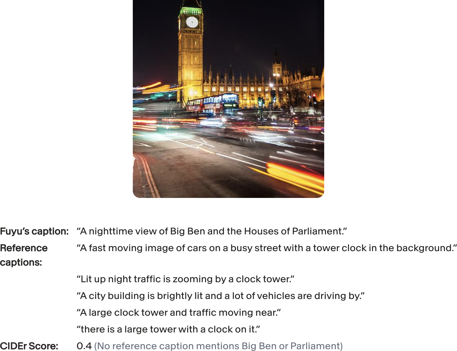
Figure 3-5. An example where Fuyu generated a correct option but was given a low score because of the limitation of reference captions.
Not only that, but references can be wrong. For example, the organizers of the WMT 2023 Metrics shared task, which focuses on examining evaluation metrics for machine translation, reported that they found many bad reference translations in their data. Low-quality reference data is one of the reasons that reference-free metrics were strong contenders for reference-based metrics in terms of correlation to human judgment (Freitag et al., 2023).
Semantic Similarity
Lexical similarity measures whether two texts look similar, not whether they have the same meaning. Consider the two sentences "What's up?" and "How are you?" Lexically, they are different—there's little overlapping in the words and letters they use. However, semantically, they are close. Conversely, similar-looking texts can mean very different things. "Let's eat, grandma" and "Let's eat grandma" mean two completely different things.
Semantic similarity aims to compute the similarity in semantics. This first requires transforming a text into a numerical representation, which is called an embedding. For example, the sentence "the cat sits on a mat" might be represented using an embedding that looks like this: [0.11, 0.02, 0.54]. Semantic similarity is, therefore, also called embedding similarity.
"Introduction to Embedding" discusses how embeddings work. For now, let's assume that you have a way to transform texts into embeddings. The similarity between two embeddings can be computed using metrics such as cosine similarity. Two embeddings that are exactly the same have a similarity score of 1. Two opposite embeddings have a similarity score of –1.
Mathematically, let be an embedding of the generated response, and be an embedding of a reference response. The cosine similarity between and is computed as , with:
Metrics for semantic textual similarity include BERTScore (embeddings are generated by BERT) and MoverScore (embeddings are generated by a mixture of algorithms).
Semantic textual similarity doesn't require a set of reference responses as comprehensive as lexical similarity does. However, the reliability of semantic similarity depends on the quality of the underlying embedding algorithm. Two texts with the same meaning can still have a low semantic similarity score if their embeddings are bad.
Before we move on to discuss AI as a judge, let's go over a quick introduction to embedding. The concept of embedding lies at the heart of semantic similarity, and is the backbone of many topics we explore throughout the book, including vector search in Chapter 6 and data deduplication in Chapter 8.
Introduction to Embedding
Since computers work with numbers, a model needs to convert its input into numerical representations that computers can process. An embedding is a numerical representation that aims to capture the meaning of the original data.
An embedding is a vector. For example, the sentence "the cat sits on a mat" might be represented using an embedding vector that looks like this: [0.11, 0.02, 0.54]. Here, I use a small vector as an example. In reality, the size of an embedding vector (the number of elements in the embedding vector) is typically between 100 and 10,000.
Models trained especially to produce embeddings include the open source models BERT, CLIP (Contrastive Language–Image Pre-training), and Sentence Transformers. There are also proprietary embedding models provided as APIs.
Table 3-2. Embedding sizes used by common models.
| Provider / Model | Variant | Embedding Size |
|---|---|---|
| Google's BERT | BERT base | 768 |
| BERT large | 1024 | |
| OpenAI's CLIP | Image | 512 |
| Text | 512 | |
| OpenAI Embeddings API | text-embedding-3-small | 1536 |
| text-embedding-3-large | 3072 | |
| Cohere's Embed v3 | embed-english-v3.0 | 1024 |
| embed-english-light-3.0 | 384 |
Because models typically require their inputs to first be transformed into vector representations, many ML models, including GPTs and Llamas, also involve a step to generate embeddings. "Transformer architecture" visualizes the embedding layer in a transformer model. If you have access to the intermediate layers of these models, you can use them to extract embeddings. However, the quality of these embeddings might not be as good as the embeddings generated by specialized embedding models.
The goal of the embedding algorithm is to produce embeddings that capture the essence of the original data. How do we verify that? The embedding vector [0.11, 0.02, 0.54] looks nothing like the original text "the cat sits on a mat".
At a high level, an embedding algorithm is considered good if more-similar texts have closer embeddings, measured by cosine similarity or related metrics. The embedding of the sentence "the cat sits on a mat" should be closer to the embedding of "the dog plays on the grass" than the embedding of "AI research is super fun".
You can also evaluate the quality of embeddings based on their utility for your task. Embeddings are used in many tasks, including classification, topic modeling, recommender systems, and RAG. An example of benchmarks that measure embedding quality on multiple tasks is MTEB, Massive Text Embedding Benchmark (Muennighoff et al., 2023).
I use texts as examples, but any data can have embedding representations. For example, ecommerce solutions like Criteo and Coveo have embeddings for products. Pinterest has embeddings for images, graphs, queries, and even users.
A new frontier is to create joint embeddings for data of different modalities. CLIP (Radford et al., 2021) was one of the first major models that could map data of different modalities, text and images, into a joint embedding space. ULIP (unified representation of language, images, and point clouds) (Xue et al., 2022) aims to create unified representations of text, images, and 3D point clouds. ImageBind (Girdhar et al., 2023) learns a joint embedding across six different modalities, including text, images, and audio.
Figure 3-6 visualizes CLIP's architecture. CLIP is trained using (image, text) pairs. The text corresponding to an image can be the caption or a comment associated with this image.
Encode each modality
For each (image, text) pair, CLIP uses a text encoder to convert the text to a text embedding, and an image encoder to convert the image to an image embedding.
Project into a joint space
It then projects both these embeddings into a joint embedding space.
Pull matching pairs together
The training goal is to get the embedding of an image close to the embedding of the corresponding text in this joint space.
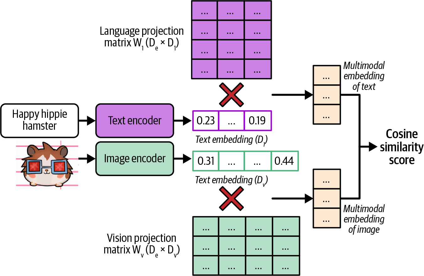
Figure 3-6. CLIP's architecture (Radford et al., 2021).
A joint embedding space that can represent data of different modalities is a multimodal embedding space. In a text–image joint embedding space, the embedding of an image of a man fishing should be closer to the embedding of the text "a fisherman" than the embedding of the text "fashion show". This joint embedding space allows embeddings of different modalities to be compared and combined. For example, this enables text-based image search. Given a text, it helps you find images closest to this text.